Ignite LocationTech Boston 2013 Wrap-Up

One of the great things about living in Boston is that there is a very active geo-community.  Every few weeks there is something interesting happening, whether it is an AvidGeo meet-up, a geo-colloquium at one of the many schools in Boston, or an industry sponsored event.

One of those events happened this past Monday at Space with a Soul in Boston’s Innovation District, organized by Avid Geo and the Eclipse Foundation’s LocationTech group.  The event focused on open source geo-based projects. The room was full of geo-thinkers from a variety of backgrounds, and thanks to a number of sponsors (AppGeo, Azavea, IBM, Actuate) there was plenty of food and beer!  Added bonus, participants from the PostGIS code sprint were in town!

The lighting talk format – five minutes, 20 slides, auto advancing – works really well for these types of events.  The speakers are energized and the crowd stays captivated.  I tried in vain to keep up with Twitter during the event.  Let’s take a look at my 140 character rundown of the evening.

Quick note – I missed a couple speaker’s names.  If you know them please post a comment so I can update accordingly. UPDATE – I only need one more name!

Second quick note- Ignore the grammar mistakes in my tweets.  I am a horrible with my thumbs.

Andrew Ross from LocationTech opened up the evening.  He talked about the mission of LocationTech and explained how the Eclipse Foundation helps open source projects get off the ground and stay relevant.

Max Uhlenhuth from SilviaTerra then gave a great overview how he started contributing to open source projects.  Max had a number of great points but a couple really stuck with me.  In his professional career he has only used open source software, and he was using FOSS in high school!  When I was in high school my parents had just gotten this new thing called the “internet.”  His best quote came about halfway through his talk:

Michael Evans and his colleague whose name escapes me (if you know, please let me know so I can update this post) talked about ongoing efforts in Boston’s City Hall to improve data sharing, analysis and visualization.  They talked about the extremely popular blizzard reporting site that famously crashed and how it was both a success and a failure.   It was a success because it was so popular, and it was a failure because it crashed, and crashed hard.  They also talked about efforts to make data resources work with more efficiency within City Hall.

I’ve seen Jeffrey Warren from the Public Laboratory give talks a few times over the past couple years and he and his colleagues are always doing something innovative.  He didn’t disappoint during his talk on Monday.  He talked about the Public Laboratory’s open source spectrometer.  It was pretty amazing.  I wish he had another 25 minutes to go into more detail.

Leaflet made an appearance at the event as well.  Calvin Metcalf, leaflet guru and cat enthusiast, gave a talk titled –Leaflet for some cats.  Using Max Ogden’s Javascript for Cats for inspiration, Calvin went through a few examples of how easy Leaflet is to use and customize.  If you haven’t tried Leaflet yet you should.  Calvin’s slides can be found here.

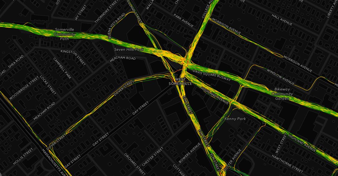
Christian Sparning from the Metropolitan Area Planning Council talked about the Hubway’s visualization hackathon.  If you are in the Boston area you have probably seen some of the results of this event over the past several months.  The Hubway folks released a whole bunch of data  – ride numbers, origin/destination data, temporal data – and then held an hackathon.  Christian talked about the variety of people who participated and the variety of creative ways they analyzed and visualized the data.

UPDATE:  Thanks to Andrew Ross I got an update on the evening’s last speaker (I didn’t catch his name at first).  The last talk was from Ken Walker from Eclipse, talking about the Orion Editor.  I’m not too familiar with Orion, which is a browser-based tool for developing on and for the web, but it looked like something I should learn about, soon.  I encourage you to check out the link to learn more.  Ken was kind enough to post his slides as well.

Overall, this was a great event.  Avid Geo and LocationTech did a great job putting this together and the speakers inspired those in the audience.  I really think you are seeing the future of geo at events like this.  Geo is no longer just for technicians working in municipal offices.  Geo is moving beyond GIS, web mapping, and cartography.  Geo is now everywhere and anywhere and that is a great thing.  In the near future geo will be even more ubiquitous throughout the business and technology worlds and there will be a growing demand for people trained in the geospatial sciences.   Events like this keep the field moving forward!

The Basics

What are our geo-analysis fundamentals?

Fundamentals should be conceptually simple, so that one can learn them and understand them quickly and easily.  Lately, three basic fundamentals of geo-analysis have been ringing in my head and I think anyone who works in “spatial” should really understand them.  Here they are, in no particular order:

If geo-analysis is your area of expertise, you should be able to discuss all three topics with some intelligence.  I know there are many more fundamentals that build the foundation of geo-analysis, but these are the three that have been thinking off lately.  Do you have any other geo-analysis fundamentals that you think are crucial to know?  If so, leave a comment.

GeoAwesome: Ignite Spatial Boston 2012

One word: GeoAwesome.  That is how I would describe tonight’s (11/14/2012, GIS Day!) Ignite Spatial Boston 4, which was organized by Avid Geo, hosted by the Center for Geographic Analysis at Harvard University and sponsored by AppGeo, Axis Maps, NBT Solutions, Azavea, and CDM Smith.  The twelve, five minute talks covered a variety of geo-topics from analysis to workflow, apps and technology.  It was a really well-rounded night of topics.  I thought all the speakers did an excellent job.  Here is a real quick rundown of the talks:

Crowdsourcing Boston’s Neighborhood Boundaries – Andy Woodruff, Axis Maps.  Great idea, great application, great participation, and great execution.  I can’t wait to see what they do next.  Check out Bostonography for more.

Save your Mouse: Automate your Spatial Workflow with PostGIS – Jesse Bishop, Research Associate, Woods Hole Research Center. You know you’re onto something when you are saving yourself literally millions of mouse clicks. Great project and great technique. Really opens up your schedule!

Visualizing the Urban Metabolism of Neighborhoods – Dr. David Quinn, urbmet.  This was one of several talks that discussed a geospatial analysis that was data intensive, innovative, and had great visualization component.  Dr. Quinn did a great job of breaking it all down in five minutes.

Trafficked by Sea – Stacy Bogan, Center for Geographic Analysis, Harvard University.  Presented a unique approach to modeling ocean traffic networks.  During her talk she proved that projections do matter!

Geeky Boating Elk, Ryan Westphal, Lead Developer, jQuery Geo Project.  Great presentation, taking a totally wild and creative subject, and using it to demonstrate the power or jQuery Geo.

GeoHOLLIS: Mapping the ILibrary Catalog – Bonnie Burns, Harvard Map Collection.  I used to work in a map library so I can really appreciate this project.  So far they have geo-cataloged 12.5% of their 12 million records, allowing patrons to search their catalog geographically.

Fontly: Mapping the World of Vintage Typography – Brendan Ciecko, Founder, Fontly.  I was really impressed with this talk.  Check out Fontly and contribute to the project.

Estimating Sandy – Ben Spaulding and Boyd Zapatka, AIR Worldwide.  My co-worker and I gave this talk about the work we have been doing the past couple weeks.  It’s amazing how much geoscience you can jam into five minutes.

Python as an ETL – Mark Zito, GIS Specialist, CDM Smith.  Mark demonstrated a few workflows using Python as a geospatial extract,transform and load tool.  I need to ask him about getting one of his code samples.

Partly Cloudy: Real World Tales of Geo Migration to AWS – Michael Terner, EVP, AppGeo.  Michael shared AppGeo’s experiences about moving to the cloud.  Really focused on the benefits, which I thought were right on the money (he talked about cost savings, if you didn’t get my pun).

Making Sense of 500 Million Location Requests Per Day – Richard Sutton, Geospatial Lead, Skyhook.  I think everyone who was in the room (100+ people) wanted his data and databases after he finished his talk.  I can’t describe how incredible the data and analysis he described are.  The potential for this data is unbelievable.

Cartographic Ingredients from the Eye Candy Kitchen – Jeff Blossom, Center for Geographic Analysis, Harvard University.  We often forget the basics that make a map a pleasure to gaze upon.  Jeff did a great job of breaking down the basic ingredients all cartographers need to remember when creating a map.

A big thanks to Guido Stein and the Avid Geo crew for bringing us this event.  There is a strong geo-community in Boston and events like this really bring it to the forefront!  

More Spatial SQL – Calculating Lines between Points

Recently I posted some tips and example script to measure distance between points using SQL Server.  The obvious extension of this script would be to generate the lines between two points. I wanted to create a script that took two points from a table and using STLineFromText to create the line. The vast majority of the script is the same as the previous post, with the exception of the line to create the lines.  So, here it is:

select 
t1.Id as ID, 
t1.NAMEASCII as t1_Name, 
t1.SOV0NAME as t1_SOV0NAME, 
t1.Latitude as t1_Latitude, 
t1.Longitude as t1_Longitude, 
t2.ID as t2_ID, t2.NAMEASCII as t2_Name, 
t2.SOV0NAME as t2_SOV0NAME, 
t2.LATITUDE as t2_Latitide, 
t2.LONGITUDE as t2_Longitude,
Geography::Point(t1.Latitude, t1.Longitude, 4326).STDistance(Geography::Point(t2.LATITUDE, t2.LONGITUDE, 4326)) as Distance_Meters,
Geography::STLineFromText('LINESTRING('+cast(cast(t1.longitude as float)as varchar)+' '+cast(cast(t1.latitude as float)as varchar)+','+cast(cast(t2.longitude as float)as varchar)+' '+cast(cast(t2.latitude as float)as varchar)+')', 4326) as line
from dbo.Populated_Places t1 cross join dbo.Populated_Places t2
where t1.SOV0NAME = 'United States' and  t2.SOV0NAME = 'United States'  and t1.ID != t2.ID and t1.NAMEASCII = 'Boston'

A few notes about this script:

  • I am using SQL Server 2008 R2.
  • Unfortunately, you cannot pass values directly into the STLineFromText method like you can other Spatial SQL methods.  When using the STLineFromText the user needs to convert the coordinate pairs into a LineString.  This isn’t that big of a deal since the LineString allows a users to string together a series of coordinate pairs to create complex line objects, which is a big plus (in this example I am creating lines between two points), I had to use a cast a couple times to get the coordinate data in the correct format.  I experimented with a couple different ideas and this one worked.  This probably isn’t the best way to do this so if you have a better idea please post a comment!
  • The line that is being generated is a geodesic line.  Why is that?  I am using the Geography data type and I am calling an SRID of 4326 when STLineFromText is executed.  The combination of the two will create “near” geodesic lines as opposed to planar lines.
  • Like in the previous post, a self cross join is being used to create the location pairs.
  • There are a couple items in the where statement that need to be mentioned.  The query above will not work if the coordinate pairs represent the same location, meaning STLineFromText cannot create a line where the two points represent the same space.  To prevent this error I simply set the query to not select IDs that are equal.  The results of this query return the distance and generates a line between all populated places in the United States from Boston.  To prove this works, here is a nice little image:

Lines between Points
Ok, that’s it.  Pretty simple and pretty fast (the example query takes two seconds to run). Perhaps I’ll put together a simple script to string together multiple points into a line or multi-line object next!

Hurricane Sandy! Data and Maps

I noticed earlier that my post about last year’s major New England storm was getting a ton of action today.  It’s probably time to get some info up about Hurricane Sandy.

I’ll keep updating this page when I come across data sets or mapping sites with pertinent information about the event.  If you have a good link post it in the comments section!

Last updated 11/4/2012

Storm Mapping Sites

Hurricane Sandy Data

Twitter/Social Media Mapping


Power Outage Sites

I’m in Somerville, Massachusetts and the wind has been whipping all day.  If the power stays on I’ll try to update this page if I come across some more data and maps.


Using a Where Statement in a SQL Spatial Join

I had a question the other day about how to incorporate a where statement into a spatial join (STIntersects).  Unfortunately, the examples I had previously posted didn’t cover that topic.  Well, here is an example of querying two tables, using the geometry data type in each, along with a where statement, to find all results that meet the defined spatial conditions:

select PP.*, SP.*
from Populated_Places PP
inner join States_Provinces SP with(Index(geom_sidx))
on PP.geom.STIntersects(SP.geom) = 1
where SP.NAME_0 = 'United States of America' 
and SP.NAME_1 = 'Massachusetts'

Let’s breakdown this query:

  • The query starts by calling all the columns from two different tables, a table with point data called Populated_Places, and a table containing polygon data called State_Provinces.
  • The query then performs an inner join between the two tables, In the inner join I specifically call the spatial index from the States_Provinces table.  I call this index because I want to use it, and because query optimizer may skip it, as it does with many spatial indexes.
  • In the ON statement I set up the STIntersects statement between the point table and the polygon table, only returning the records that intersect.  This is done by setting the Boolean requirement at the end of the STIntersects statement to 1.  I also make sure to set the correct column in each table that contains the spatial  datatype, which in this case is called geom for both tables.
  • Now, here comes the where statement,which is about as vanilla as vanilla can be.  In the where statement I simply limit the polygons that are eligible for the query based on some defined values.

This type of query will also work with line or polygon features, as demonstrated in the following picture.  In this example I query all the roads that intersect a polygon defined in the where statement.  You will notice that I have the spatial results tab open to display the intersecting line features.

This is a pretty simple example, but if you have never worked in this medium it can be a little confusing at first.  Have any more spatial sql questions?  Let me know.  I need to keep sharp.

The First Law of Geography – Today’s Geo Inspiration

Ever now and then I look for inspiration when designing a model or writing some code to solve a geo-problem.  Recently, while searching for some geo-inspiration I came across one of my favorite papers.  If you have ever taken any type of  GIS or spatial analysis course you have probably heard some variation of the following phrase, commonly referred to as the First Law of Geography:

“Everything is related to everything else,
but near things are more related than distant things”

This idea, my friends, is what defines the field of geo-analysis.  From interpolation to distance decay, and spatial autocorrelation to gravity models, the idea that locations that are closer together are more related than those that are far apart provides the base for the field of geographic analysis.  Like any great quote, many may know it but few know it’s origins.  So, where did this phrase come from?  Here it is…

A Computer Movie Simulating Urban Growth in the Detroit Region
W. R. Tobler
Economic Geography
Vol. 46, Supplement: Proceedings. International Geographical Union. Commission on Quantitative Methods (Jun., 1970), pp. 234-240

Waldo Tobler is very well known geographer (he has his own Wikipedia page!) and if you have ever taken a geography or GIS course at some point the professor probably referred to his work, either directly or indirectly.  A copy of the paper is available here and a reply to the First Law of Geography can be found here.  If you are in the learning mood both are quick reads.

Geospatial Topology, the Basics

The concept of topology isn’t something that every spatially enabled person fully understands.  That is OK, because I too had to learn (and relearn) how spatial topology works over the years, especially early on back in the ArcView 3.X days.  I think this experience is fairly typical of someone who uses GIS.  If one is taking a GIS course or a course that uses GIS it is not very often that the concept of spatial topology is covered in-depth or at all.  Spatial topology also may not be something that people are overly concerned about during their day-to-day workflow, meaning they may let their geospatial topology skills slide from time to time.  As a public service here is a basic overview of geospatial topology.

First question: What is topology?

You have probably heard the term topology before, whether it was in a GIS course where the instruction lightly glazed over the topic, or in a geometry/mathematics course.

Technically speaking, topology is a field of mathematics/geometry/graph theory, that studies how the properties of a shape remain under a number of different transformations, like bending, stretching, or twisting.   The field of topology is well established within mathematics and far more complicated than I wish to get in this post.

Second question: How does topology relate to GIS and spatial analysis?

Spatial analysis is at its core an analysis of shapes in space.  Geospatial topology is used to determine and preserve the relationships between shapes in the vector data model.

The GIS software we use for analysis and data storage incorporates a set of “topological rules” to define how vector objects are stored and how they can interact with each other.  These rules can dictate how nodes interact within a network, how the edges or faces of polygons coexist, or how points are organized across space.

Back in the “olden-days” (which was before “my time”) GIS users, particularly ArcInfo users, were well versed in geospatial topology because of the coverage.  The coverage data model, a precursor to today’s ubiquitous shapefile format, was unique in that topology was stored within the file.  This data format allowed users a certain set of controls to the spatial relationships within the dataset that later went away with the shapefile.  The shapefile is not a topologically valid dataset, as geometric relationships are not enforced.  For example, how may of you have downloaded (or bought) a shapefile from a data provider and it was FULL of slivers? In the Esri world geospatial topology came back with the geodatabase, and has been incorporated into a number of other geospatial data formats including spatial databases supported by Oracle, PostGIS (2.0) and SpatiaLite.

Today, topology is important in geodatabase design (for those who pay attention to it!), and data creation/editing.  By understanding the set of geospatial topology rules and creating topologically sound data, the user can have a level of trust in their data during analysis.

 Additional Resources:

Esri white paper on GIS topology 

PostGIS Topology

PostGIS 2.0 Topology Support

Oracle Topology Data Model

Vector topology in GRASS

Esri Coverage Topology

Esri Geodatabase Topology

Real topology

Vector topology cleaning with Quantum and GRASS – youtube vid

GISDoctor Spatial Analysis Post Series

There once was a well know GIS blog post that compared geographic information systems to word processors.  No matter what you think about the post we will always need people who are skilled at “writing” and have something to “write” about.

As I have said before, and will say again, if you are using GIS technologies you should have a grasp on the fundamentals.  You wouldn’t write a paper or a report without a grasp on the basics of the topic or without a knowledge of writing in general.  So, to improve the world’s GIS grammar (or at least my own), I will be posting a number of spatial analysis related topics over the course of the next few months.  Here are a few of the topics I will cover:

  • Data classification schemes
  • Understanding spatial random samples
  • Topology, from a spatial point of view
  • The basics of projections
  • Avoiding false accuracy
  • Using root mean square
  • Geary’s c and Moran’s I
  • The First Law of Geography
  • Spatial autocorrelation
  • and many more…

I’ll use a variety of software, data, and problems to explain these topics, in order to expose the reader to the broad language of GIS.